Below are descriptions of some of my data science projects. You can also click on the titles for links to the code on github.

Recommendation system for rock climbing routes

mountainproject.com is a website that provides information about rock climbing areas and allows users to rate climbing routes. Using data that I scraped from Mountain Project, I built a collaborative-filter recommender system that recommends new routes in The Shawangunks (Gunks) in upstate New York. I also built a climbing partner finder that pairs climbers based on their climbing preferences.

I examined 470 routes in the Gunks which were rated by about 2,400 climbers for a total of about 31,000 ratings.

Climbing routes can be rated from 0-4 and the mean rating is 2.9. About half of the climbers have rated 5 or fewer routes.

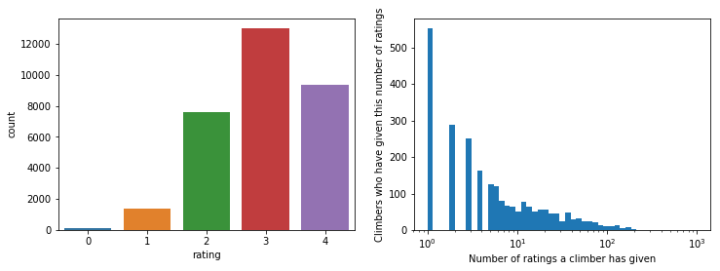
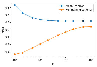
Using the collaborative-filtering library surprise, I trained a k-nearest neighbor estimator to predict the ratings that climbers would give to routes they have not climbed yet. This can then be used to rank the top N climbs to suggest to each climber. The root-mean-square error (RMSE) for the final model was 0.62. This can be compared to the baseline RMSE of 0.87 that I get if I just use the average rating of all climbing routes.

5-fold cross validation of a user-based k-nearest neighbor estimator. The value k=500 neighbors minimizes the root-mean-squared cross-validation error. 

In addition, the k-nearest neighbors works by calculating the similarity between climbers (for a user-based similarity calculation) or the similarity between climbing routes (for an item-based similarity calculation). This allows us to suggest climbing partners by ranking climbers that are most similar. Or, if a climber is looking for new routes that are most like a given route, the item-based similarity can suggest the most similar routes. Examples of these rankings can be found in this notebook.

Predicting Rossmann store sales

Rossmann is a European drug store chain based in Germany. Using a dataset for the daily sales in each of ~1000 stores over approximately three years, I built a model that can predict daily sales in each store 6 weeks in advance. This was part of a Kaggle competition. Below is an example of the predicted sales for my model compared with the actual sales in one of the stores.

Training set (top) and validation set (bottom) for sales in Rossmann store #1. True sales are blue, predicted sales from the Random Forest Regressor are green, and the residuals (errors) are red.

There are two main components that predict the sales in a store. The first is the averaged past history for each store. The second is periodic trends that depend on the day of the week, the day of the month, and the month.

Daily sales compared to the mean sales averaged over 3 years.

Periodic components for the daily sales. There is clear dependence on the day of the week, day of the month, and month.

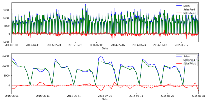
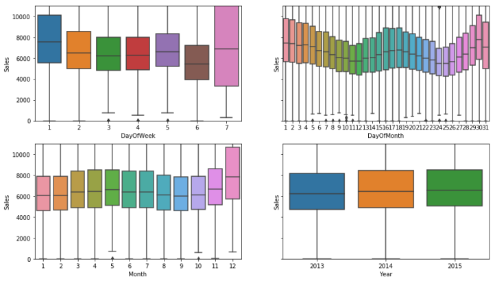
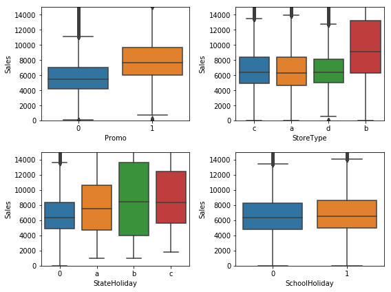
In addition, there are other quantities that predict the sales such as a promotion on a given day, the layout of the store, and whether or not a given day is a state holiday or school holiday.

Daily sales for each store split up according to promotion, store type, state holiday, and school holiday.

I trained a Random Forest Regressor using these features (as well as a couple others). To do this, I broke up the data into a training set, and left out the last 2 months as a validation set. I chose the hyperparameters of the Random Forest model that minimized the fractional RMSE on the validation set. I was able to a achieve a RMSE of 13.5%. The current best score is 10%.

Ranking loans from Lending Club

Using a dataset from the peer-to-peer lending company Lending Club, I built a model to predict the expected ROI on unsecured 3-year personal loans. With this model I then made a recommender that ranks borrowers within a grade based on their expected ROI so that lenders can invest in the most profitable loans.

There were several parts to the process:

1. Data cleaning: This involved selecting features such as loan purpose, home ownership, income, and past delinquencies, and removing any features that were not available at the time the loan was issued. I then performed imputation on missing data and one-hot-encoding for categorical data.
2. Predict defaults: I used a random forest classifier to predict if a borrower would default. Because only 8%-17% of borrowers default, the data set is imbalanced. I therefore used the F1 score which balances precision and recall to optimize the random forest hyperparameters.
3. Calibrate default probability: As a result of the data imbalance, the classifier’s probability estimator massively underestimates the actual frequency of defaults for a test-set. So, I recalibrated the probability estimator.
4. Estimate recovery of defaulted loans: For loans that do default, lenders will still be able to recover some of the owed amount. I performed regression to estimate the fraction of the loan that would be recovered. After trying multiple algorithms (e.g. linear regression, support vector regression, random forests) I found that none of them were were accurate than simply predicting the mean recovered value of 42%, so I concluded that there was very little information left in the data, and just used the mean value.
5. Predict ROI: With the calibrated model for default probability and the model for recovery of defaulted loans I then calculated the expectation value for the total amount paid back. This can then be translated to an annualized rate of return. With this the available loans can be ranked, and investors can choose the most profitable loans.

Tutorial on regression techniques

I made this tutorial on regression techniques using scikit-learn for a workshop on Reduced Order Gravitational-Wave Modeling held in June 2018. It covers linear models (Ridge, Lasso), kernel techniques (Kernel Ridge, Support Vector Regression, Gaussian Process Regression), Neural Networks, and tree-based fitting (Random Forest). The goal was to demonstrate regularization and cross-validation methods that let the data choose the complexity of the model.

As an example, let’s look at Ridge regression. Below are 10 data points produced by adding a small error to a known function shown in red.

The true function and 10 data points with small errors.

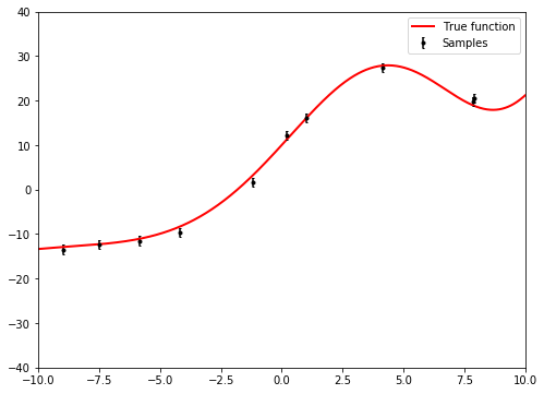
We want to fit this data with a parameterized function, and a standard function to try is a polynomial:

.

If we think of each power as a new feature in a high dimensional space, we can treat this as just an n-dimensional linear model:

.

We can find the coefficients in this model by minimizing a cost function given by the average squared difference between the model and the data :

.

However, the standard question is: which order polynomial do we choose? If we choose a low order polynomial, the function won’t have enough complexity to accurately fit the data. If we choose a high order polynomial, the function will be overfit and won’t generalize to new data. As an example, below is an 11th order polynomial (12 free coefficients) fit to the 10 data points. The system is technically underdetermined and clearly overfits the data

11th order polynomial fit to the 10 data points.

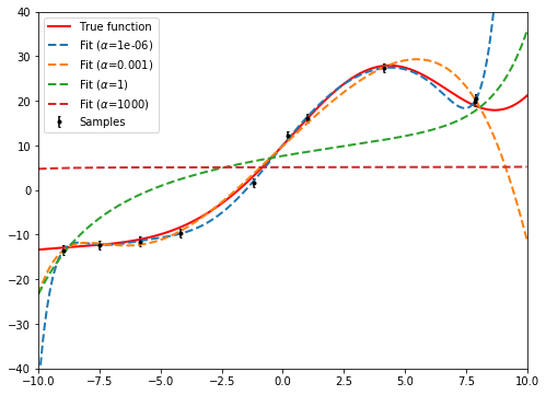
Instead of using a lower order polynomial to avoid overfitting, we can instead place a penalty on the size of coefficients resulting in a simpler fitting function. This method is known as regularization. The cost function that is minimized has an additional term for the coefficients, and looks like

.

The larger the hyperparameter , the smaller the coefficients that minimize the cost function. (Note that when using regularization, it is necessary to scale all features so that they have similar numerical values. In the notebook on github, all features in the training set were rescaled to lie in the range [0, 1].)

For small values of α, the size of the coefficients is not limited, and the fitting function can be complex. However, as α increases, large coefficients are disfavored, and the fitting function becomes simpler.

The optimal value of the hyperparameter can be chosen with k-fold cross-validation. The steps are as follows:

1. Break the data into k sets.
2. Fit the function with k-1 (training) sets. Calculate the error with the other (validation) set.
3. Cycle through the sets so that each set is the validation set exactly once.
4. Choose the hyperparameters that give the smallest average error for the validation set.
5. Retrain on the entire training set with the chosen hyperparameters.

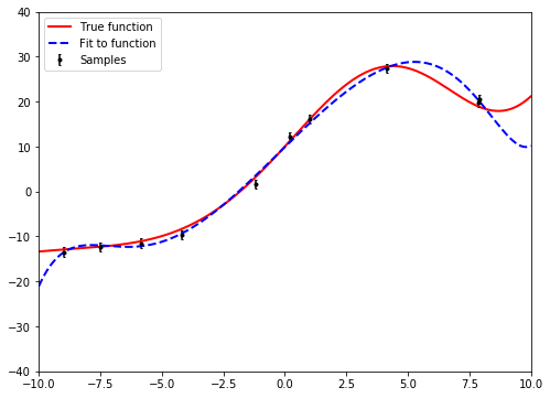
Below is the fitting function after the optimal value of is chosen.

The value α=0.0007 minimized the cross-validation error.

Predicting the sale prices of homes

The goal of this project is to predict the sale prices of houses in Ames, Iowa using a training set of sale prices and about 80 features of each house. I obtained a fractional RMSE of 14%. The current best score is 11%.

I converted categorical features (e.g. ‘foundation type’ and ‘neighborhood name’) to binary features with one-hot-encoding, and ordinal features (e.g. exterior quality ratings {‘Poor’: 1, ‘Fair’: 2, ‘TA’: 3, ‘Good’: 4, ‘Excellent’: 5}) to numerical rankings. I imputed missing data to appropriate values depending on the context.With the cleaned, numerical data, I split the data into a training set and validation set. I examined several regression algorithms (Ridge, Lasso, Kernel Ridge, Support Vector Regression, Decision Tree, Random Forest, Neural Network). After optimizing the hyperparameters of each algorithm to minimize the 10-fold cross-validation error for the training set, I chose the model with the lowest error on the final validation set. This happened to be Support Vector Regression with a radial basis function kernel.

10-fold cross-validation error for Support Vector Regression with a radial basis function kernel as a function of the hyperparameters (penalty C and scale factor γ). The values that minimize this error were chosen for the final model.